High-Performance Computing

UP

The numerical solution of complex problems in engineering requires a huge amount of computational resources. Today's largest supercomputers provide a performance of 10-100 PFlops/sec and we are entering the era of Exascale computing in the near future (probably in the next decade), see TOP500 list for recent developments. While previous progress in compute hardware has been mainly related to improvements in the single core performance (e.g., frequency), modern supercomputers in the so-called "post-frequency" era will be characterized by massive parallelism with several millions of compute cores. The development of software tools (see for example the SPPEXA project) targeting these recent developments in compute hardware is of outmost importance to fully exploit the compute capabilities of future HPC systems. Apart from the requirement of the scalability of algorithms to millions of processors, writing software that makes efficient use of modern cached-based architectures on the single core or single node level is the very first and most important step in high-performance computing. Hence, the main aspects to be addressed regarding the development of high-performance PDE solvers are the following:

to identify the bottleneck that limits compute performance,
to characterize algorithms into memory-bound and compute-bound algorithms,
to efficiently use the available memory bandwidth (DRAM gap) as well as caches,
to utilize the SIMD capabilities of modern compute hardware (AVX2, AVX512) in case of compute-bound algorithms,
to exploit intra-node parallelism of modern multicore CPUs, and
to target the massive parallelism of large supercomputers by efficient parallelization techniques.

Our research focuses on the developement of generic, high-performance implementations of high-order continuous and discontinuous Galerkin finite element methods. From an application point of view, we put an emphasis on developing high-performance methods in the fields of incompressible flows and especially turbulent incompressible flows where engineering applications are very demanding in terms of computational costs.

Example of performance modeling

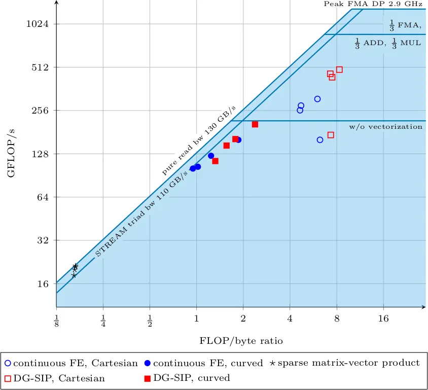
The following figure shows a roofline performance model of various code patterns developed at the Institute for Computational Mechanics under the lead of Dr. Martin Kronbichler, measured on a node of 2x14 cores of Intel Broadwell (Xeon E5-2690 v4) running at 2.9 GHz. Each setup is ran for four polynomial degrees, k=1, 3, 5, 9. The roofline model is a well-established performance model and plots the achieved arithmetic throughput (measured as GFLOP/s) over the arithmetic intensity of the kernel, i.e., the number of floating point operations performed for each byte loaded from main memory. The model is based on the observation that either the throughput from main memory is the limiting factor (diagonal lines in the plot) or the actual compute performance (horizonal lines). The upper horizonal line at 1.3 TFLOP/s is the peak arithmetic performance when only doing floating point fused multiply-add (FMA) instructions, which are advertised by computer manufacturers as the most relevant metric in the LINPACK benchmark (large dense matrix factorization). However, for realistic codes, the bar is lower. For our DG codes, the appropriate upper limit is the second horizontal line because the instruction mix of floating point operations involves approximately 35% FMAs, 30% additions or subtractions, and 35% multiplications.

The figure shows the performance of the evaluation of the Laplacian. Classical sparse-matrix based kernels (stars on the lower left of the picture) are completely bound by the available bandwidth from RAM memory, not by compute throughput. Our matrix-free kernels based on sum factorization significantly reduce the memory access and thus increase throughput. The implementation automatically detects simple meshes such as Cartesian ones, in which case the memory access is lowered considerably and the arithmetic balance shifts to the right. Due to the optimized implementation, most of the data points are still in the memory limited regime once advanced implementation techniques such as SIMD vectorization are applied. Our research regarding algorithm development is guided by this roofline or more advanced models such as the execution cache memory (ECM) model that can also explain parts of the gap for the Cartesian-mesh cases.

Example of typical code patterns - SIMD vectorization

As mentioned above, arithmetically intense kernels profit from the CPU's vector units that can perform several arithmetic operations within a single instruction (SIMD). Our implementation framework in C++ makes extensive use of the available units.

Here is an example of the machine code (assembler code, AT&T sytnax) from an inner loop from our sum factorization kernels that are underlying the high-order discontinuous Galerkin implementations, vectorized with the recent AVX-512 instruction set extension for Intel Xeon Phi Knights Landing or Xeon Scalable (Skylake-X), for a polynomial degree of 6. Note that the implementation is done in high level (templated) C++ code with operator overloading and reasonably nice user interfaces, whereas the code shown here is the final output of an optimizing compiler (first column: address within the instruction stream, second column: binary machine code in hex format, third column: human-readable assembler commands).

  424170:    62 f1 fd 48 28 40 06     vmovapd 0x180(%rax),%zmm0 
  424177:    62 f1 fd 48 28 08        vmovapd (%rax),%zmm1
  42417d:    48 05 c0 01 00 00        add    $0x1c0,%rax 
  424183:    48 81 c1 c0 01 00 00     add    $0x1c0,%rcx 
  42418a:    62 f1 fd 48 28 50 fa     vmovapd -0x180(%rax),%zmm2 
  424191:    62 f1 fd 48 28 58 fb     vmovapd -0x140(%rax),%zmm3 
  424198:    62 f1 fd 48 28 60 fc     vmovapd -0x100(%rax),%zmm4 
  42419f:    62 61 f5 48 58 d8        vaddpd %zmm0,%zmm1,%zmm27 
  4241a5:    62 f1 f5 48 5c c8        vsubpd %zmm0,%zmm1,%zmm1 
  4241ab:    62 f1 fd 48 28 40 fe     vmovapd -0x80(%rax),%zmm0 
  4241b2:    62 f1 fd 48 29 61 fc     vmovapd %zmm4,-0x100(%rcx) 
  4241b9:    62 61 ed 48 58 e0        vaddpd %zmm0,%zmm2,%zmm28 
  4241bf:    62 f1 ed 48 5c d0        vsubpd %zmm0,%zmm2,%zmm2 
  4241c5:    62 f1 fd 48 28 40 fd     vmovapd -0xc0(%rax),%zmm0 
  4241cc:    62 61 e5 48 58 d0        vaddpd %zmm0,%zmm3,%zmm26 
  4241d2:    62 f1 e5 48 5c c0        vsubpd %zmm0,%zmm3,%zmm0 
  4241d8:    62 21 9d 40 59 e8        vmulpd %zmm16,%zmm28,%zmm29 
  4241de:    62 b1 ed 48 59 da        vmulpd %zmm18,%zmm2,%zmm3 
  4241e4:    62 02 9d 48 b8 eb        vfmadd231pd %zmm27,%zmm12,%zmm29 
  4241ea:    62 f2 95 48 b8 d9        vfmadd231pd %zmm1,%zmm13,%zmm3 
  4241f0:    62 42 ad 40 b8 eb        vfmadd231pd %zmm11,%zmm26,%zmm29 
  4241f6:    62 b2 fd 48 b8 df        vfmadd231pd %zmm23,%zmm0,%zmm3 
  4241fc:    62 62 c5 48 b8 ec        vfmadd231pd %zmm4,%zmm7,%zmm29 
  424202:    62 01 e5 48 58 f5        vaddpd %zmm29,%zmm3,%zmm30 
  424208:    62 f1 95 40 5c db        vsubpd %zmm3,%zmm29,%zmm3 
  42420e:    62 21 9d 40 59 ec        vmulpd %zmm20,%zmm28,%zmm29 
  424214:    62 f1 fd 48 29 59 ff     vmovapd %zmm3,-0x40(%rcx) 
  42421b:    62 b1 ed 48 59 de        vmulpd %zmm22,%zmm2,%zmm3 
  424221:    62 61 fd 48 29 71 f9     vmovapd %zmm30,-0x1c0(%rcx) 
  424228:    62 02 a5 40 b8 e9        vfmadd231pd %zmm25,%zmm27,%zmm29 
  42422e:    62 b2 f5 48 b8 d9        vfmadd231pd %zmm17,%zmm1,%zmm3 
  424234:    62 42 ad 40 b8 ef        vfmadd231pd %zmm15,%zmm26,%zmm29 
  42423a:    62 f2 fd 48 b8 de        vfmadd231pd %zmm6,%zmm0,%zmm3 
  424240:    62 62 ad 48 b8 ec        vfmadd231pd %zmm4,%zmm10,%zmm29 
  424246:    62 01 e5 48 58 f5        vaddpd %zmm29,%zmm3,%zmm30 
  42424c:    62 f1 95 40 5c db        vsubpd %zmm3,%zmm29,%zmm3 
  424252:    62 f1 fd 48 29 59 fe     vmovapd %zmm3,-0x80(%rcx) 
  424259:    62 f1 ed 48 59 dd        vmulpd %zmm5,%zmm2,%zmm3 
  42425f:    62 61 fd 48 29 71 fa     vmovapd %zmm30,-0x180(%rcx) 
  424266:    62 91 9d 40 59 d0        vmulpd %zmm24,%zmm28,%zmm2 
  42426c:    62 b2 f5 48 b8 dd        vfmadd231pd %zmm21,%zmm1,%zmm3 
  424272:    62 42 ed 48 98 d8        vfmadd132pd %zmm8,%zmm2,%zmm27 
  424278:    62 d2 e5 48 98 c1        vfmadd132pd %zmm9,%zmm3,%zmm0 
  42427e:    62 91 fd 48 28 cb        vmovapd %zmm27,%zmm1 
  424284:    62 b2 ad 40 b8 cb        vfmadd231pd %zmm19,%zmm26,%zmm1 
  42428a:    62 f2 8d 48 b8 cc        vfmadd231pd %zmm4,%zmm14,%zmm1 
  424290:    62 f1 fd 48 58 d1        vaddpd %zmm1,%zmm0,%zmm2 
  424296:    62 f1 f5 48 5c c0        vsubpd %zmm0,%zmm1,%zmm0 
  42429c:    62 f1 fd 48 29 51 fb     vmovapd %zmm2,-0x140(%rcx) 
  4242a3:    62 f1 fd 48 29 41 fd     vmovapd %zmm0,-0xc0(%rcx) 
  4242aa:    48 39 c6                 cmp    %rax,%rsi 
  4242ad:    0f 85 bd fe ff ff        jne    424170

Scaling on SuperMUC

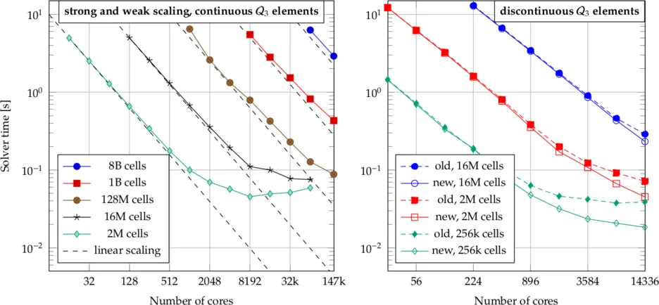
The left panel of the following picture shows a scaling experiment on up to the full Phase 1 of SuperMUC consisting of up to 9216 nodes with 2x8 core Intel Xeon E5-2680 at 2.7 GHz. Along each line, the problem size is held constant as the number of processors increases (strong scaling). Furthermore, there are several lines of successively larger problems, indicating also the weak scalability of our implementation. The plot shows absolute solution times to a tolerance of 1e-9 with a geometric multigrid preconditioner inside a conjugate gradient iterative solve. The largest problem involves 8 billion cells of continuous cubic interpolations on the Laplacian, i.e., 232 billion degrees of freedom.

The right panel shows a scaling plot that contains some improvements for the multigrid implementation that have been derived by our group, running experiments on SuperMUC Phase 2 on up to 14,336 cores. It can clearly be seen that the latency at larger processor counts has been significantly improved by the implementation labeled 'new' in the figure.